Understanding how to measure market efficiency is a major concern for investors and business owners.
Investors are interested in the efficiency of a market because the level of a market’s efficiency is one of the determinants of the price of investments and the possible returns on the investments.
Business owners are equally concerned with market efficiency because it determines the volatility or stability of assets as it ensures one of the most accurate valuations and pricing of assets.
Before we discuss how to measure market efficiency, let us understand the meaning of an efficient market.
Read about: Examples of Efficient Market Hypothesis
What is an efficient market?
An efficient market refers to a market where all information about assets is transmitted perfectly, completely, instantly, and without additional cost.
This implies that whenever a piece of new information that may affect the prices of assets in a financial market comes about, everyone receives the entire information.
It also implies the prompt distribution of the information as well as the absence of fees or any other forms of payment before accessing such information. Thus, efficient markets are characterized by high liquidity, low transaction costs, and a high degree of transparency.
Due to the accurate incorporation of all available information in the pricing of assets in an efficient market, it is extremely difficult for investors to achieve consistent returns above the market average through active trading strategies or analysis of publicly available information.
This supports the efficient market hypothesis which asserts that securities such as stocks, bonds, and commodities are traded at their intrinsic values, hence limiting arbitrage opportunities or undervalued assets.
Read about: Weak Form Efficient Market Hypothesis
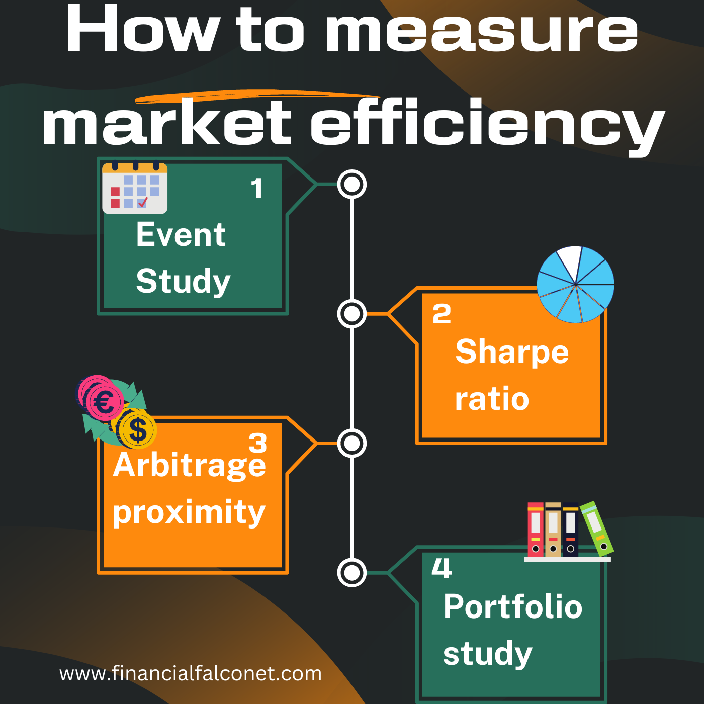
Measures of market efficiency
- Event study
- Sharpe ratio
- Arbitrage proximity
- Portfolio study
Measuring market efficiency through event study
This measure of market efficiency is designed to examine how the market reacts to events and excess returns associated with such events.
The events can vary from firm-specific events such as mergers, acquisitions, and dividend announcements, to market-wide events such as macro-economic announcements.
When using an event study to measure market efficiency, a cross-section of the market is usually used. This is done to eliminate bias by ensuring adequate market representation and to have a clear result that shows if the market is efficient or not.
An event study is usually carried out using the following steps:
1. Identify the event and the specific date of announcement
Identifying the event to be studied and the specific announcement date is important because financial markets generally react to announcements on the occurrence of certain events rather than the event itself.
This is so because, in most instances, announcements are made days, weeks, or even months ahead of the event.
For instance, before shareholders get paid dividends, the company will declare dividends and announce in advance, the date when the dividends will be paid out.
2. Track returns for the period under review
The returns gained on assets within the specified period are tracked in a bid to ascertain if there are changes. When tracking returns, it can be hourly, daily, weekly, or monthly.
The frequency of returns tracking is usually determined by how precise the event announcement is, the interval between the time of the announcement and the event, and how quickly new information is reflected in the price of the assets.
Generally, the more precise the announcement, the easier it is to track the returns using shorter intervals. And the faster the adjustments of price to event announcements, the higher the possibility of using shorter tracking intervals.
Based on the aforementioned, the event window to be tracked, which comprises the period before the announcement and after the event needs to be clearly stated.
This is mathematically expressed as R-n……….R0……….R+n
where
R-n = returns for the period before the announced event date
R0 = returns on the event date
R+n = returns for the period after the event
Thus the overall return (R) for the event window will be a combination of all the returns from period R-n, through R0, to R+n. This is done for all the companies in the sample.
For instance, if a company makes an announcement in March 2024, about a merger that will occur in May 2024, the event window for this announcement can be a few days before the announcement and a few days after the date of the announcement.
This means the returns for each of these days within the event window will be tracked to note if there are changes in the returns due to the announcement.
The precision of the event date usually determines the lengthiness or shortness of the event window. The more imprecise the date, the longer the event window; the more precise the date, the shorter the event window.
3. Adjust the tracked returns for market performance and risk.
The returns that have been tracked during the event window have to be adjusted for market performance and risks to arrive at the excess returns. This is done for all the companies in the sample.
For example, suppose you use the capital asset pricing model (CAPM) to control for risk. In that case, the excess return for each company can be arrived at by subtracting the sum of the risk-free rate and the beta market return within the period under review from the overall return during the event window.
This can be expressed as ER = R – (Riskfree rate + Beta return on market for the period) where
ER = Excess returns during the event window
R = Overall return during the event window
4. Compute the standard error
After all the excess returns for the sample companies have been compiled and the average for the period under review, a standard error is computed. This is expressed as follows:
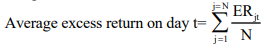
where ER =Excess returns
N = Number of events in the study
5. Estimate the T statistic
The T statistic for each day of the event is estimated by dividing the average excess return by the standard error to determine if the excess returns around the announcement are different from zero.
If the T statistics are significant at 2.55 and 1.96 for a 1% or 5% significance level respectively, then it shows that the event affects returns.
The sign of the excess return, whether positive or negative will determine if the effect of the event on returns is positive or negative.
Sharpe ratio
The Sharpe ratio can be used to test the efficiency of a market that has a finite number of assets within a specified period. The assets may be individual assets or a group of assets such as investment portfolios.
The ratio is obtained by dividing the difference between the expected return and the risk-free return rate by the standard deviation of the investment. This is mathematically expressed as:
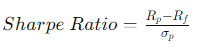
Where Rp = Expected return of the investment
Rf = Risk-free return rate
Rσ = Standard deviation of the investment returns
Generally, the smaller the value of an investment’s Sharpe ratio, the more efficient the market whereas a large Sharpe ratio value indicates an inefficient market.
A market with a Sharpe ratio between 0 and 1 is considered efficient whereas a market with values above 1 is considered inefficient.
Arbitrage proximity
Arbitrage proximity is one of the easiest measures of market efficiency. When markets are efficient, the prices of assets reflect all available information which implies the correct valuation of assets.
This means that the price of an asset such as the stocks of a company will be traded at the same price on different exchanges. If this is so, it eliminates the possibility of investors gaining through arbitrage trading.
Hence, when a market has little or no arbitrage proximity, it indicates that the market is efficient. Markets with large arbitrage proximity on the other hand are inefficient.
Measuring market efficiency using portfolio study
In a bid to outperform the market, some investors build investment portfolios with assets that share similar characteristics. This strategy aims to gather undervalued assets that are likely to earn higher than market average returns for the owner.
To test the efficacy of this investment strategy as well as the market efficiency, the portfolio study is used.
The portfolio study is based on observable characteristics of the companies whose stocks are contained in the portfolio that are traded in a particular market. These observable characteristics include price-to-earnings (PE) ratios, dividend yields, price-to-book value ratios, etc.
The study creates a portfolio of investments with similar characteristics which are traced over time to ascertain the efficiency or inefficiency in the portfolio. The steps involved in the portfolio study include:
1. Identify the observable characteristic
This is the first step in carrying out a test for market efficiency using the portfolio study. The observable characteristics can be the stock price, price-to-book value ratio, market value of the equity, etc.
2. Group the companies
The companies are classified group into different portfolios based on the similarities in traits. For example, if the stock price is the observable characteristic that is tracked, all companies whose stock price falls within the range of $5 to $10 can be grouped whereas those whose stock price ranges between $100 to $120 can be grouped.
The number of companies in each portfolio will depend on the overall sample size used in the study. Each portfolio must have a good number of companies to ensure the result is accurate.
Collate the data
Data on the selected observable characteristic is collected for all the companies that are part of the market efficiency test.
3. Calculate the return for each portfolio
The individual returns are collected and then the return for each portfolio is calculated. The assumption when calculating the portfolio return, especially when using stock price as the observable characteristic is that the stocks are equally weighted.
4. Estimate the beta for each portfolio
The beta or betas of each portfolio are estimated. When only a single factor is used in the study i.e., the single factor model, the beta of the portfolio is calculated. If a multifactor model is used, i.e. comparing several observable characteristics, the betas of the portfolio are calculated.
The beta is calculated by regressing the portfolio’s return against market returns for a specified period; usually a year before the testing period or by taking the average beta of the individual stocks in the portfolio.
5. Calculate the excess returns
The excess returns earned by each portfolio are computed alongside the standard error of the excess returns. Statistical tests such as parametric or nonparametric tests are used to check whether the average excess returns are different across the portfolios.
Parametric tests usually test for equality across the portfolios while nonparametric tests rank up returns across the portfolios and then sum the ranks within each group to check whether the rankings are random or systematic.
6. Check for differences
Finally, the extreme portfolios can be matched against each other to see whether there are statistically significant differences across these portfolios.
Read about: Assumptions of the Efficient Market Hypothesis (EMH)
How to measure market efficiency
Measuring market efficiency aids investors make better decisions on which markets to invest in, as it presents them with factual information on how much returns they could make on their investments.
Companies may also consider a market’s efficiency before listing their stocks in order to ensure they get prized appropriately. Below are the steps taken when measuring market efficiency.
Define the market and assets
The first step when measuring market efficiency is to define the market and the assets that will be tested for efficiency. This is necessary because markets can vary in size, scope, complexity, and the assets therein.
Identify the information
Identify the types of information relevant to the market and assets under consideration. This could include fundamental data such as financial statements and economic indicators; technical data such as price and volume trends; or insider information.
Develop your hypothesis
Formulate the specific hypotheses or assertions about the efficiency of the market that you want to test. This could be how past price movements do not predict future price movements, the effects of stocks being included in an index, etc.
Choose methodology
Select appropriate methodologies for testing your hypothesis. This could involve statistical tests, portfolio studies, econometric models, or event studies. The choice of methodology depends on the nature of the data and the hypothesis being tested.
Collect relevant data
Gather relevant data that aligns with the particular hypothesis you are testing. The data collected may include historical data on market prices, trading volumes, company financials, and economic indicators. Ensure the data is accurate, reliable, and covers a sufficiently long period to analyze market behavior.
Analyze the data
Analyze the collected data using the chosen methodology. Evaluate whether the empirical evidence supports or contradicts the efficiency hypothesis that was proposed earlier. This could involve assessing the significance of correlations, conducting regression analyses, or comparing actual market behavior to theoretical expectations.
Interpret results
Interpret the result of the data analysis in the context of the efficiency hypothesis being tested. Determine whether the market exhibits efficiency characteristics or if the evidence indicates inefficiency.
Conclusion and documentation
Draw conclusions based on the findings of the analysis. Determine the degree to which the market is efficient or inefficient according to the evidence gathered.
Document the research methodology, results, and conclusions in a straightforward manner. This aids future research on market efficiency.
In addition, communicate findings to relevant stakeholders, such as investors, regulators, or academic peers, through reports, presentations, or publications.
Read about: Criticism of Efficient Market Hypothesis (EMH)
Examples of measures of market efficiency
Example of event study
An event study can be used to examine the effect of option listing on the stock price. For a long time, there have been arguments suggesting that option listing increases stock price volatility by attracting speculators.
On the other hand, others argue that option listing increases the available choices for investors and the flow of information to financial markets thereby leading to lower stock price volatility and higher stock prices.
To test these alternative hypotheses, Jennifer Conrad carried out an event study in 1989 to understand the effect of option introduction on the underlying stock price.
The steps used in carrying out the study are as outlined in the event study that was discussed earlier. The table below summarizes the findings from Conrad’s study.
| Trading day | Average excess return | Cumulative excess return | T statistic |
|---|---|---|---|
| -10 | 0.17% | 0.17% | 1.30 |
| -9 | 0.48% | 0.65% | 1.66 |
| -8 | -0.24% | 0.41% | 1.43 |
| -7 | 0.28% | 0.69% | 1.62 |
| -6 | 0.04% | 0.73% | 1.62 |
| -5 | -0.46% | 0.27% | 1.24 |
| -4 | -0.26% | 0.01% | 1.02 |
| -3 | -0.11% | -0.10% | 0.93 |
| -2 | 0.26% | 0.16% | 1.09 |
| -1 | 0.29% | 0.45% | 1.28 |
| 0 | 0.01% | 0.46% | 1.27 |
| 1 | 0.17% | 0.63% | 1.37 |
| 2 | 0.14% | 0.77% | 1.44 |
| 3 | 0.04% | 0.81% | 1.44 |
| 4 | 0.18% | 0.99% | 1.54 |
| 5 | 0.56% | 1.55% | 1.88 |
| 6 | 0.22% | 1.77% | 1.99 |
| 7 | 0.05% | 1.82% | 2.00 |
| 8 | -0.13% | 1.69% | 1.89 |
| 9 | 0.09% | 1.78% | 1.92 |
| 10 | 0.02% | 1.80% | 1.91 |
Based on the result, it was discovered that the introduction of individual options causes a permanent price increase in the underlying security, beginning approximately three days before introduction.
It was also observed that the price effect was not on the announcement day alone but throughout the event window. Thus, the event study supports the argument that option listing enhances market efficiency by increasing the flow of information to financial markets which leads to lower stock price volatility and higher stock prices.
Example of Sharpe ratio
Assuming a passive index fund has an annual return of 12%, a 20% standard deviation of returns, and a 4% risk-free rate, we can calculate the Sharpe ratio thus:
Sharpe ratio = 12% – 4% / 20%
Sharpe ratio = 8% / 20%
Sharpe ratio = 0.40
If over the years the Sharpe ratio for the index fund remains at 0.40 or drops lower, the market can be assumed to be efficient. If however the Sharpe ratio increases and goes above 1, it means the market has become less efficient with time.
Arbitrage proximity
Arbitrage proximity takes advantage of differences in prices in different markets to make a profit. For example, if a company’s stock sells for $5 on exchange A and sells for $7 on exchange B, an investor can buy such from exchange A and sell it simultaneously on exchange B to make a $2 profit.
When the market is efficient, the stock will sell for the same price on both exchanges A and B. In a situation where there will be a price difference, it will be very low such as between $0.1 – $0.5
Portfolio study
Investors generally assert that stocks with low price-earnings ratio do much better than stocks with high price to earnings ratios. To test this hypothesis, firms on the New York Stock Exchange (NYSE) were grouped into 5 in 1987 based on their price-earnings ratio.
The first group consisted of stocks with the lowest PE ratios and the fifth group consisted of stocks with the highest PE ratios. From 1988 to 1992, the returns on each portfolio were computed for 5 years. Stocks in the portfolio that went bankrupt or were delisted were assigned a return of -100%.
The portfolios were assumed to be equally weighted and the average beta for each portfolio was computed.
The returns on the market index as well as the excess returns on each portfolio were computed.
| P/E Class | 1988 | 1989 | 1990 | 1991 | 1992 | 1988 – 1992 |
|---|---|---|---|---|---|---|
| Lowest | 3.84% | -0.83% | 2.10% | 6.68% | 0.64% | 2.61% |
| 2 | 1.75% | 2.26% | 0.19% | 1.09% | 1.13% | 1.56% |
| 3 | 0.20% | -3.15% | -0.20% | 0.17% | 0.12% | -0.59% |
| 4 | -1.25% | -0.94% | -0.65% | -1.99% | -0.48% | -1.15% |
| Highest | -1.74% | -0.63% | -1.44% | -4.06% | -1.25% | -1.95% |
Based on the result, the ranking of the returns across the portfolio classes seems to confirm the hypothesis that stocks with low price to earnings ratio earn a higher return compared to those with high PE ratios.
We have to however consider whether the differences across portfolios are statistically significant. This can be done using an F test to accept or reject the hypothesis that the average returns are the same across all portfolios. A high F score would lead us to conclude that the
differences are too large to be random.
Read about: Types of Efficient Market Hypothesis (EMH)
How do you test market efficiency?
You can test for market efficiency by using a portfolio approach, event study, arbitrage proximity, or Sharpe ratio. The particular method used varies based on the choice of the individual carrying out the test, the type of assets sold in the market, and the investment scheme being tested.
Conclusion
Several methods such as event study and Sharpe ratio are used in testing market efficiency. Arbitrage proximity and portfolio study are additional measures of market efficiency.
In a 2017 study carried out by Madan et al., they concluded that in equity markets, efficiency is enhanced when up moves are more frequent and smaller in size than their downside counterparts. This is the property of markets taking escalators up and elevators down.
For commodity markets the opposite is the case. For currencies, the results are mixed depending on the choice of the quoting currency. The property is however prevalent for USD as the quoting currency.

Blessing's experience lies in business, finance, literature, and marketing. She enjoys writing or editing in these fields, reflecting her experiences and expertise in all the content that she writes.